Building a Construction Site Safety Monitor with YOLOv12

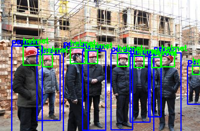
Construction sites are among the most hazardous work environments, with head injuries accounting for a significant portion of workplace accidents. Ensuring consistent compliance with safety protocols remains a challenge for site managers who must monitor large areas and numerous workers simultaneously.

In this tutorial, we’ll build an automated safety monitoring system using YOLOv12, the latest version of the popular YOLO (You Only Look Once) object detection model. Our system will detect whether construction workers are wearing hard hats, providing a practical solution for real-time safety compliance monitoring.

Why This Matters

Traditional safety monitoring relies on manual inspection by supervisors, which is:

• Time-consuming: One supervisor can only monitor a limited area

• Inconsistent: Human attention fluctuates throughout the day

• Reactive: Violations are often caught after the fact

An automated computer vision system can:

• Monitor multiple camera feeds simultaneously

• Provide real-time alerts when violations are detected

• Generate compliance reports automatically

• Free up supervisors to focus on other critical tasks

What We’ll Build

By the end of this tutorial, you’ll have a working system that can:

1. Detect people in construction site images

2. Identify whether each person is wearing a helmet

3. Classify workers as “compliant” (wearing helmet) or “non-compliant” (no helmet)

4. Visualize the results with bounding boxes and labels

Prerequisites

Before we begin, you should have:

• Basic Python programming knowledge

• Familiarity with Jupyter notebooks or Google Colab

• Understanding of basic machine learning concepts (training, validation, testing)

• A Roboflow account (free tier works fine)

No prior experience with YOLO or computer vision is required, we’ll explain everything as we go.

Project Overview

Our approach involves three main steps:

1. Dataset preparation: Download and organize a dataset of construction workers with labeled hard hats

2. Model training: Fine-tune a pre-trained YOLOv12 model on our specific dataset

3. Safety monitoring: Combine helmet detection with person detection to identify compliance violations

1. Setting Up the Environment

All the code in this guide can be access on this Colab Notebook.

First, we need to install the required libraries. We’ll use:

• Roboflow: For downloading our pre-labeled dataset

• Ultralytics: The official library for YOLO models

!pip install roboflow ultralytics -q

Next, import all necessary libraries:

from roboflow import Roboflow
import yaml
from ultralytics import YOLO
from PIL import Image
import matplotlib.pyplot as plt
import os, random, shutil
from glob import glob
from collections import Counter
import matplotlib.patches as patches
import matplotlib.image as mpimg
import cv2

2. Downloading the Dataset

We’ll use Roboflow’s Hard Hat Workers dataset, which contains images of construction workers labeled with two classes:

• Head: A person’s head without a helmet

• Helmet: A person’s head with a hard hat

• Person: A Person (We won’t be using this label for this task)

rf = Roboflow(api_key="YOUR-ROBOFLOW-API-KEY")

project = rf.workspace("joseph-nelson").project("hard-hat-workers")
version = project.version(2)
dataset = version.download("yolov12")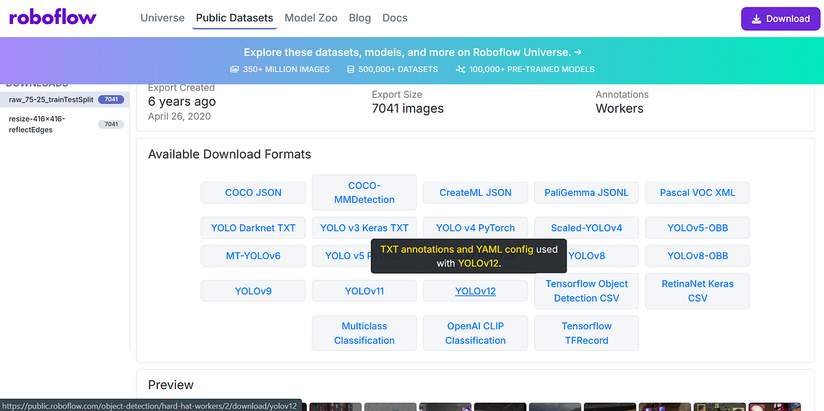

Note: Replace the API key with your own from Roboflow. You can get one by clicking on the YOLOv12 option in the dataset page. A dialog will popup with an option to show download code. Copy this code and replace the code above with it.

This code:

1. Connects to Roboflow using your API key

2. Accesses the “hard-hat-workers” project

3. Downloads version 2 of the dataset in YOLOv12 format

Let’s verify the download and see what we got:

data_dir = dataset.location

print("Dataset downloaded to:", dataset.location)
os.listdir(data_dir)

Output:

Dataset downloaded to: /content/Hard-Hat-Workers-2
['README.dataset.txt', 'README.roboflow.txt', 'test', 'data.yaml', 'train']

You should see folders named train , and test along with a data.yaml configuration file.

3. Understanding the Dataset Structure

YOLO models expect data in a specific format:

• Images folder: Contains .jpg or .png files

• Labels folder: Contains .txt files with the same names as images

• data.yaml: Configuration file specifying paths and class names

Each label file contains one line per object in the format:

class_id x_center y_center width height

All coordinates are normalized (between 0 and 1) relative to the image dimensions.

4. Updating the Configuration File

The data.yaml file contains this information:

train: ../train/images
val: ../valid/images
test: ../test/images

nc: 3
names: ['head', 'helmet', 'person']

roboflow:
  workspace: joseph-nelson
  project: hard-hat-workers
  version: 2
  license: Public Domain
  url: https://universe.roboflow.com/joseph-nelson/hard-hat-workers/dataset/2

The first two 3 lines point to our train, valid and test sets. The actual dataset, however, does not have the valid set, so we are going to create it in the next steps.

Additionally, the person class is underrepresented in both train and test sets with only 615 labels compared to 19747 for the helmet class and 6677 for the head class across the two sets combined.

Let’s update the data.yaml file to ensure that we only use the head and helmet classes in our training:

yaml_path = os.path.join(data_dir, "data.yaml")

# Load the existing YAML
with open(yaml_path, "r") as f:
    data = yaml.safe_load(f)

# Update only the relevant keys
data["nc"] = 2
data["names"] = ["head", "helmet"]

# Save the changes
with open(yaml_path, "w") as f:
    yaml.dump(data, f, default_flow_style=False)

# Confirm the new YAML contents
!cat "$yaml_path"

This ensures our model knows:

• nc = 2: We have 2 classes

• names: Class 0 is “head”, class 1 is “helmet”

5. Creating a Validation Set

Machine learning models need three datasets:

• Training set: Used to teach the model

• Validation set: Used to tune hyperparameters and prevent overfitting

• Test set: Used for final evaluation

Our downloaded dataset has train and test sets, but we need to create a validation set from the training data:

train_dir = os.path.join(data_dir, "train")
test_dir = os.path.join(data_dir, "test")
valid_dir = os.path.join(data_dir, "valid")

Now let’s split off 15% of the training data for validation:

# Create validation folders
os.makedirs(os.path.join(valid_dir, "images"), exist_ok=True)
os.makedirs(os.path.join(valid_dir, "labels"), exist_ok=True)

# Get all training images
train_images = glob(os.path.join(train_dir, "images", "*.jpg"))

# Define split ratio
val_ratio = 0.15
val_count = int(len(train_images) * val_ratio)

# Randomly pick validation images
val_images = random.sample(train_images, val_count)

# Move selected images and labels
for img_path in val_images:
    label_path = img_path.replace("images", "labels").replace(".jpg", ".txt")
    dest_img = img_path.replace("train", "valid")
    dest_label = label_path.replace("train", "valid")
    shutil.move(img_path, dest_img)
    if os.path.exists(label_path):
        shutil.move(label_path, dest_label)

print(f"Created validation set with {val_count} images")
print(f"Remaining training images: {len(glob(os.path.join(train_dir, 'images', '*.jpg')))}")

Output:

Created validation set with 790 images
Remaining training images: 4479

This code:

1. Creates folders for validation images and labels

2. Randomly selects 15% of training images

3. Moves both the images and their corresponding labels to the validation folder

6. Analyzing Class Distribution

It’s important to check if our dataset is balanced. If one class has far more examples than another, the model might become biased.

# Function to count class instances in a label folder
def count_labels(labels_dir):
    counts = Counter()
    for file in os.listdir(labels_dir):
        if file.endswith(".txt"):
            with open(os.path.join(labels_dir, file), "r") as f:
                lines = f.readlines()
            counts.update([int(line.split()[0]) for line in lines])
    return counts

# Paths to label folders
train_labels = os.path.join(data_dir, "train/labels")
test_labels =os.path.join(data_dir, "test/labels")
val_labels = os.path.join(data_dir, "valid/labels") if os.path.exists(os.path.join(data_dir, "valid/labels")) else None

# Count instances
train_counts = count_labels(train_labels)
test_counts = count_labels(test_labels)
val_counts = count_labels(val_labels) if val_labels else None

# Map class IDs to names
class_names = ["head", "helmet"]
print("Training set label distribution:")

for i, name in enumerate(class_names):
    print(f"{name}: {train_counts.get(i,0)} instances")

print("\nTest set label distribution:")

for i, name in enumerate(class_names):
    print(f"{name}: {test_counts.get(i,0)} instances")

if val_counts:
    print("\nValidation set label distribution:")
    for i, name in enumerate(class_names):
        print(f"{name}: {val_counts.get(i,0)} instances")

Output:

Training set label distribution:
head: 4232 instances
helmet: 12644 instances

Test set label distribution:
head: 1803 instances
helmet: 4863 instances

Validation set label distribution:
head: 642 instances
helmet: 2240 instances

This function:

1. Opens each label file

2. Counts how many times each class ID appears

3. Reports the distribution for each dataset split

7. Visualizing the Distribution

Let’s create a bar chart to see the class distribution at a glance:

# Prepare data for plotting
splits = ["train", "test", "val"]
counts = [
    [train_counts.get(0,0), train_counts.get(1,0)],  # train: head, helmet
    [test_counts.get(0,0), test_counts.get(1,0)],    # test: head, helmet
    [val_counts.get(0,0), val_counts.get(1,0)] if val_counts else [0,0]  # val: head, helmet
]

class_names = ["head", "helmet"]
bar_width = 0.35
x = range(len(splits))

# Plotting
plt.figure(figsize=(8,5))
plt.bar([p - bar_width/2 for p in x], [c[0] for c in counts], width=bar_width, label="head")
plt.bar([p + bar_width/2 for p in x], [c[1] for c in counts], width=bar_width, label="helmet")
plt.xticks(x, splits)
plt.ylabel("Number of Instances")
plt.title("Label Distribution per Split")
plt.legend()
plt.show()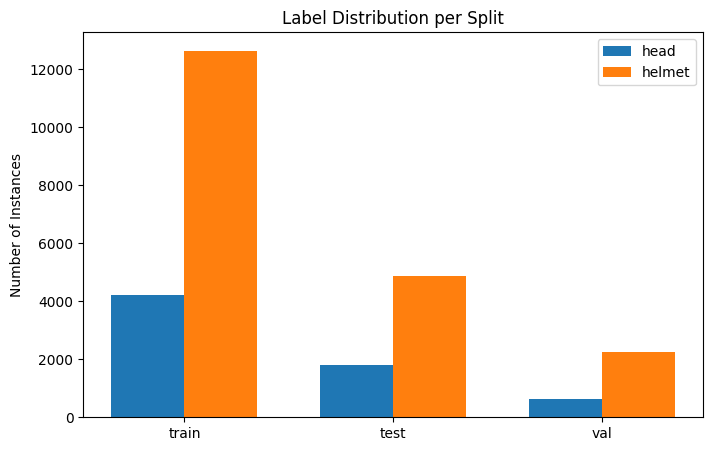

Ideally, you want roughly similar numbers for both classes to avoid bias. A small imbalance (say, 60/40) is usually fine. This particular dataset is biased with the head class having less labels than the helmet class.

8. Visualizing Sample Images with Annotations

Let’s see what our labeled data actually looks like:

# Paths
train_images_dir = os.path.join(data_dir, "train/images")
train_labels_dir = os.path.join(data_dir, "train/labels")

# Class names and colors
class_names = ["head", "helmet"]
class_colors = ["cyan", "magenta"]  # head: cyan, helmet: magenta

# Randomly select images
sample_images = random.sample(os.listdir(train_images_dir), 4)
plt.figure(figsize=(12, 10))
for i, img_file in enumerate(sample_images):
    img_path = os.path.join(train_images_dir, img_file)
    label_file = os.path.join(train_labels_dir, img_file.replace(".jpg", ".txt").replace(".png", ".txt"))

    # Load image
    img = Image.open(img_path)
    w, h = img.size

    # Plot image
    ax = plt.subplot(2, 2, i + 1)
    ax.imshow(img)

    # Load and draw labels if they exist
    if os.path.exists(label_file):
        with open(label_file, "r") as f:
            lines = f.readlines()
        for line in lines:
            class_id, x_center, y_center, bw, bh = map(float, line.strip().split())

            # Convert YOLO format to absolute box coordinates
            x = (x_center - bw/2) * w
            y = (y_center - bh/2) * h
            width = bw * w
            height = bh * h
            rect = patches.Rectangle(
                (x, y), width, height, linewidth=2, edgecolor=class_colors[int(class_id)], facecolor='none'
            )
            ax.add_patch(rect)
            ax.text(x, y-5, class_names[int(class_id)], color=class_colors[int(class_id)], fontsize=10, weight='bold')
    ax.axis("off")
plt.tight_layout()
plt.show()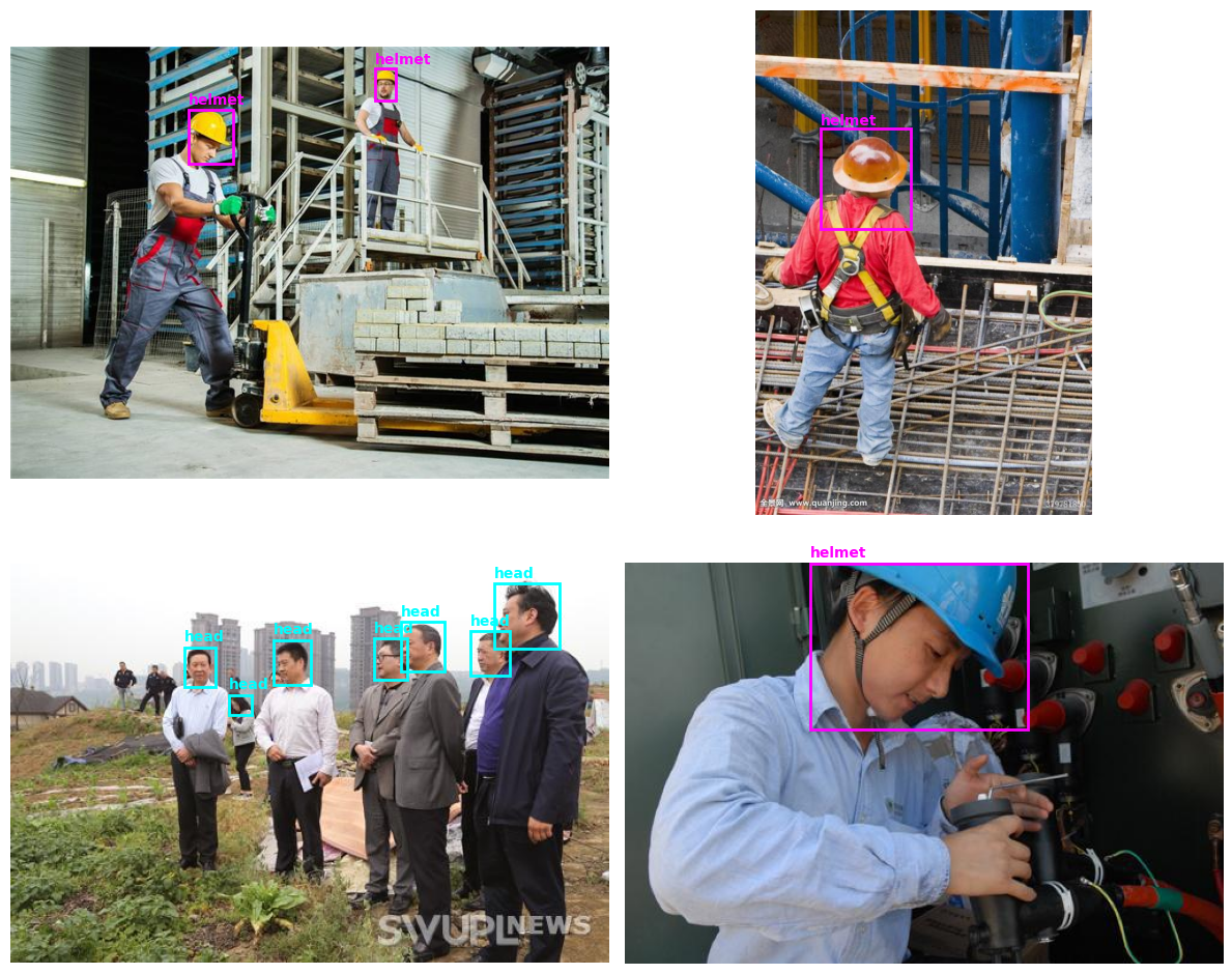

This visualization:

1. Randomly selects 4 training images

2. Draws bounding boxes around detected objects

3. Labels each box with its class name

4. Uses different colors for different classes (cyan for heads, magenta for helmets)

This helps verify that the annotations are correct before investing time in training.

9. Loading a Pre-trained Model

Instead of training from scratch, we’ll use transfer learning, starting with a model pre-trained on COCO (a large general-purpose dataset) and fine-tuning it on our specific task.

We select the smallest version of the model for our task, YOLO12n . This is to allow for faster training, but the accuracy will not be as high as when using the larger version YOLO12x which will be slower to train. Feel free to select the model that meets your needs.

# Load a pretrained YOLOv12n model (COCO pretrained)
model = YOLO("yolo12n.pt")

YOLO offers several sizes that you can explore on the Ultralytics Site for YOLO12:

• Nano (n): Fastest, good for real-time applications

• Small (s): Balanced speed and accuracy

• Medium (m): Higher accuracy

• Large (l) and Extra-large (x): Best accuracy, slower

10. Testing the Pre-trained Model

Let’s see how the model performs before training on our dataset. We select one image for this test:

# Run inference on one image
image_path = os.path.join(data_dir, "train/images/000001_jpg.rf.fddb09e33a544e332617f8ceb53ee805.jpg")
results = model(image_path, show=False)

# Visualize the results
plt.imshow(results[0].plot())
plt.axis("off")
plt.show()

Since the model is pre-trained on COCO (which includes “person” class but not “helmet” or “head”), it likely won’t detect our specific classes yet. This is expected, we need to fine-tune it!

11. Training the Model

Now for the exciting part, training our model! This process will take the pre-trained YOLOv12 weights and adapt them to recognize hard hats and bare heads.

# Train on your custom dataset
results = model.train(
    data=os.path.join(data_dir, "data.yaml"),
    epochs=50,
    imgsz=640,
    batch=16,
    name="yolov12n-hardhat",
    pretrained=True
)

Let’s break down these parameters:

• data: Path to our data.yaml configuration file

• epochs=50: The model will see the entire training dataset 50 times. More epochs can improve accuracy but may lead to overfitting

• imgsz=640: Images will be resized to 640×640 pixels. Larger sizes may improve accuracy but require more memory

• batch=16: Process 16 images at once. Larger batches train faster but need more GPU memory. Reduce this if you get out-of-memory errors

• name: A name for this training run. Results will be saved in runs/detect/yolov12n-hardhat/

• pretrained=True: Start with pre-trained COCO weights (transfer learning)

What Happens During Training?

The training process:

1. Forward pass: Images go through the model, which predicts bounding boxes and class labels

2. Loss calculation: The model’s predictions are compared to the true labels

3. Backward pass: The model adjusts its internal parameters to reduce the loss

4. Repeat: This happens for every batch in every epoch

Training 50 epochs might take about 90 minutes if training on T4 GPU runtime on Google Colab.

After training these are the validation results I got:

 Class     Images  Instances      Box(P          R      mAP50  mAP50-95)
   all        756       2760      0.942      0.923      0.965      0.687
  head        129        634      0.922       0.91      0.952      0.678
helmet        695       2126      0.962      0.937      0.978      0.696

12. Analyzing Training Results

After training completes, YOLO automatically generates a results visualization:

# Path to your training results image
img = mpimg.imread("runs/detect/yolov12n-hardhat/results.png")

plt.figure(figsize=(12, 6))
plt.imshow(img)
plt.axis("off")
plt.show()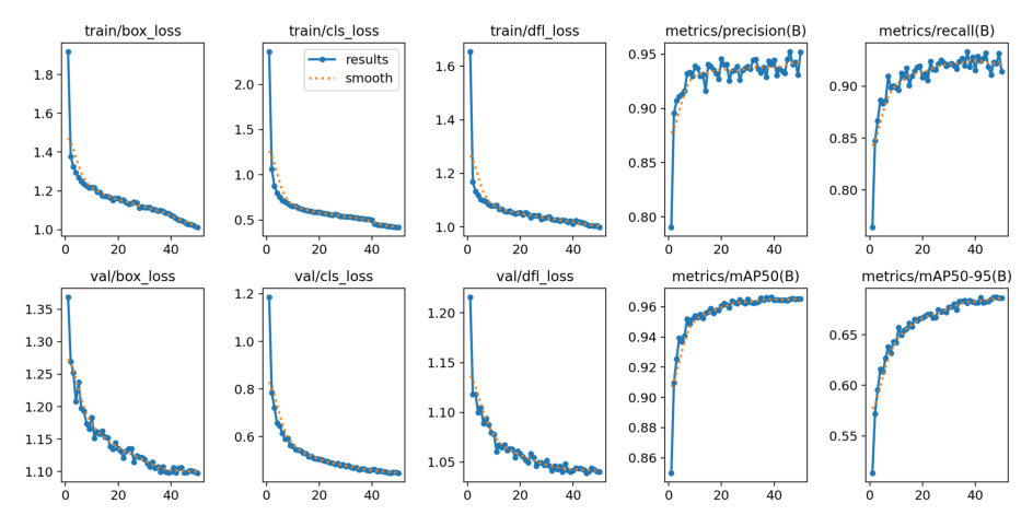

This image contains several important plots:

1. Training and validation losses: Should decrease over time

2. Precision and Recall: Should increase over time

3. mAP@0.5 and mAP@0.5:0.95: Overall performance metrics

What to look for:

• Decreasing loss: Both training and validation losses should go down

• Converging metrics: If metrics plateau, the model has learned as much as it can

• Overfitting signs: If training loss decreases but validation loss increases, you’re overfitting (model memorizing rather than learning)

13. Evaluating on the Test Set

Now let’s see how well our trained model performs on the test set — data it has never seen before:

# Load the best trained model
model = YOLO("/content/runs/detect/yolov12n-hardhat/weights/best.pt")

# Evaluate on test set
metrics = model.val(data=os.path.join(data_dir, "data.yaml"), split="test")
metrics.results_dict

Output:

 Class     Images  Instances      Box(P          R      mAP50  mAP50-95)
   all       1721       6523      0.944      0.936      0.973      0.685
  head        333       1793      0.928      0.936      0.964      0.678
helmet       1559       4730      0.961      0.937      0.981      0.692

The best.pt file contains the weights from the epoch with the best validation performance.

Key metrics to understand:

Precision: Of all detections the model made, how many were correct?

• High precision = few false positives

Recall: Of all actual objects, how many did the model find?

• High recall = few missed detections

mAP@0.5: Average precision at 50% IoU (Intersection over Union) threshold

• Good baseline metric

mAP@0.5:0.95: Average precision across multiple IoU thresholds

• More stringent metric, better reflects real-world performance

For a safety application, high recall is critical — we don’t want to miss workers without helmets!

14. Running Predictions

Let’s test our model on the entire test set and visualize some results:

# Run on an entire folder
model.predict(source=os.path.join(data_dir, "test/images"), save=True, conf=0.5)

Parameters:

• source: Folder containing test images

• save=True: Save annotated images to disk

• conf=0.5: Only show detections with 50% confidence or higher

Results are saved to runs/detect/predict/ by default.

15. Visualizing Predictions

pred_dir = "/content/runs/detect/predict"
images = [os.path.join(pred_dir, img) for img in os.listdir(pred_dir) if img.endswith((".jpg", ".png"))]

plt.figure(figsize=(14, 10))
for i, img_path in enumerate(random.sample(images, min(4, len(images)))):
    img = mpimg.imread(img_path)
    plt.subplot(2, 2, i + 1)
    plt.imshow(img)
    plt.title(os.path.basename(img_path))
    plt.axis("off")
plt.tight_layout()
plt.show()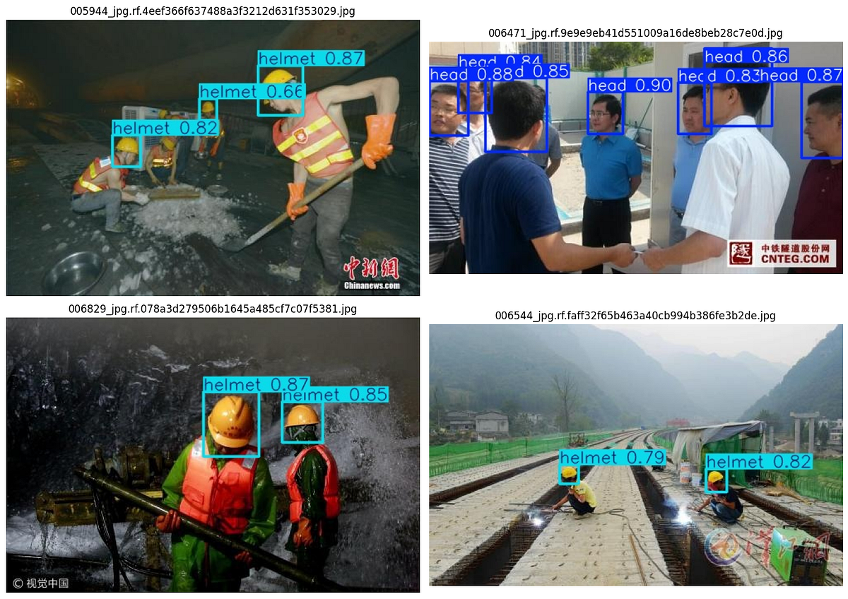

This displays 4 random predictions with bounding boxes and labels drawn on the images.

What to look for:

• Are bounding boxes tight around objects?

• Are class labels correct?

• Are there missed detections (false negatives)?

• Are there false detections (false positives)?

16. Building a Safety Compliance System

Detecting helmets and heads is useful, but for a real safety system, we need to:

1. Detect people in the scene

2. Check if each person is wearing a helmet

3. Flag non-compliant workers

This requires combining two models:

• Person detector: Detects people we’ll use the pre-trained YOLOv12 models for this. I specifically selected the bigger model YOLO12x for this part for accurate detection of people in a scene. I could also have fine-tuned this version but I didn’t due to resource constraints.

• Helmet detector: Our fine-tuned model

# Load both models
helmet_model = YOLO("/content/runs/detect/yolov12n-hardhat/weights/best.pt")
person_model = YOLO("yolo12x.pt")  # Larger model for better person detection

17. Matching People to Helmets

The key challenge is determining if a detected helmet “belongs” to a detected person. We’ll use a spatial overlap metric:

def intersection_over_helmet_area(person_box, helmet_box):
    # Compute intersection
    xi1 = max(person_box[0], helmet_box[0])
    yi1 = max(person_box[1], helmet_box[1])
    xi2 = min(person_box[2], helmet_box[2])
    yi2 = min(person_box[3], helmet_box[3])

    inter_width = max(0, xi2 - xi1)
    inter_height = max(0, yi2 - yi1)
    intersection_area = inter_width * inter_height
    
    # Helmet area
    h_width = helmet_box[2] - helmet_box[0]
    h_height = helmet_box[3] - helmet_box[1]
    helmet_area = max(1, h_width * h_height)
    return intersection_area / helmet_area

This function calculates what percentage of a helmet’s bounding box overlaps with a person’s bounding box. If the overlap is high (>30%), we consider that person to be wearing the helmet.

Why this approach?

• Helmets should always be on or near the person’s head

• If a helmet significantly overlaps with a person’s bounding box, they’re likely wearing it

• This is more robust than trying to match based on proximity alone

18. Processing Images for Compliance

Now let’s put it all together:

# Randomly select test images
N = 4
test_images = [os.path.join(data_dir, "test/images", f)
               for f in os.listdir(os.path.join(data_dir, "test/images")) if f.endswith((".jpg", ".png"))]
sample_images = random.sample(test_images, N)

processed_images = []
for img_path in sample_images:
    img = cv2.imread(img_path)
    img_rgb = cv2.cvtColor(img, cv2.COLOR_BGR2RGB)

    # Detect persons
    person_results = person_model(img_rgb, conf=0.5, classes=[0])[0]
    person_boxes = person_results.boxes.xyxy.cpu().numpy() if len(person_results.boxes) > 0 else []

    # Detect helmets
    helmet_results = helmet_model(img_rgb, conf=0.5)[0]
    helmet_boxes = helmet_results.boxes.xyxy.cpu().numpy() if len(helmet_results.boxes) > 0 else []
    with_helmet = []
    without_helmet = []
    for p_box in person_boxes:
        helmet_threshold = 0.3
        has_helmet = any(
            intersection_over_helmet_area(p_box, h_box) > helmet_threshold
            for h_box in helmet_boxes
        )
        if has_helmet:
            with_helmet.append(p_box)
        else:
            without_helmet.append(p_box)

    # Draw person boxes (blue) with label
    for p_box in person_boxes:
        x1, y1, x2, y2 = map(int, p_box)
        cv2.rectangle(img, (x1, y1), (x2, y2), (255, 0, 0), 2)
        cv2.putText(img, "person", (x1, y1-5), cv2.FONT_HERSHEY_SIMPLEX, 0.6, (255,0,0), 2)

    # Draw helmet boxes (green) with label
    for h_box in helmet_boxes:
        x1, y1, x2, y2 = map(int, h_box)
        cv2.rectangle(img, (x1, y1), (x2, y2), (0, 255, 0), 2)
        cv2.putText(img, "helmet", (x1, y1-5), cv2.FONT_HERSHEY_SIMPLEX, 0.6, (0,255,0), 2)

    # Store results
    processed_images.append((img, len(person_boxes), len(with_helmet), len(without_helmet)))

This code:

1. Runs person detection (class 0 in COCO is “person”)

2. Runs helmet detection with our fine-tuned model

3. For each person, checks if they overlap with any helmet

4. Classifies each person as compliant or non-compliant

5. Draws colored bounding boxes (blue for persons, green for helmets)

19. Visualizing Compliance Results

Finally, let’s display the results with compliance statistics:

plt.figure(figsize=(14, 10))
for i, (img, people_count, helmet_count, nohelmet_count) in enumerate(processed_images):
    ax = plt.subplot(2, 2, i+1)
    ax.imshow(cv2.cvtColor(img, cv2.COLOR_BGR2RGB))
    ax.axis("off")
    ax.set_title(f"Total People: {people_count} \nWith Helmet: {helmet_count} \nNo Helmet: {nohelmet_count}", fontsize=12)

plt.tight_layout()
plt.show()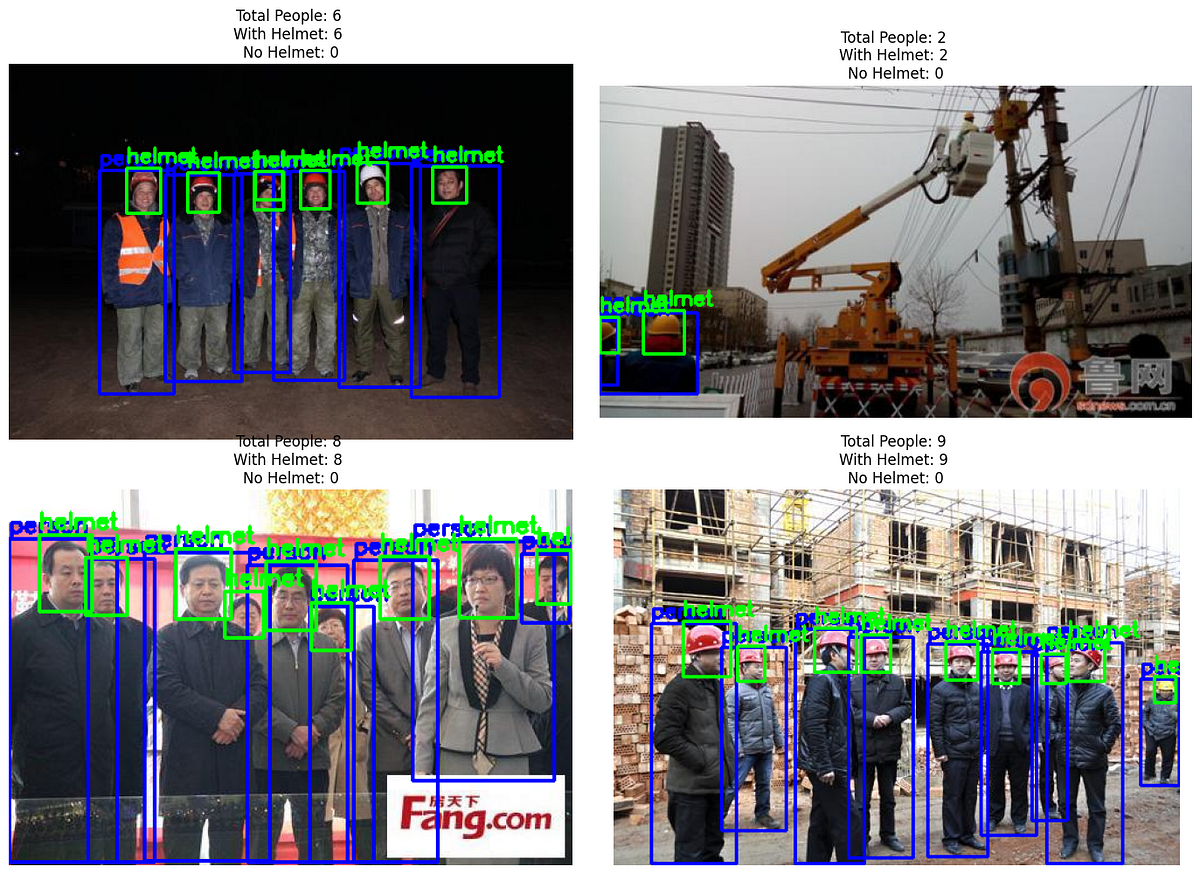

Each image shows:

• Blue boxes: Detected people

• Green boxes: Detected helmets

Title statistics:

• Total people found

• How many are wearing helmets (compliant)

• How many are not wearing helmets (violation!)

Frame 3 of our compliance results show false detection of helmets where heads are falsely detected as helmets. This highlights the limitations of our model that due to class imbalances, using a smaller model and a limited dataset.

Conclusion

Congratulations! You’ve built a complete construction site safety monitoring system. Here’s what we accomplished:

1. Downloaded and prepared a labeled dataset of construction workers

2. Explored the data to understand class distributions and verify annotations

3. Fine-tuned YOLOv12 on our custom hard hat dataset

4. Evaluated performance using standard metrics

5. Built a compliance system that detects violations in real-time

Real-World Deployment Considerations

To deploy this system in production, consider:

• Camera placement: Position cameras to capture workers’ heads clearly

• Lighting conditions: Train on images from different times of day

• Alert system: Integrate with notification systems for real-time alerts

• False positive handling: Set appropriate confidence thresholds to balance sensitivity and specificity

• Privacy: Blur faces or use only bounding boxes in stored footage

• Performance: Use a more powerful GPU or optimize the model for edge devices

Next Steps

To improve this system further, you could:

1. Collect more data: Especially for edge cases (partially visible helmets, unusual angles)

2. Experiment with model sizes: YOLOv12-s or YOLOv12-m might improve accuracy

3. Tune hyperparameters: Try different learning rates, batch sizes, or augmentation strategies

4. Add more classes: Detect other PPE like safety vests, goggles, or gloves

5. Implement tracking: Use object tracking to follow workers across video frames

6. Build a dashboard: Create a web interface for real-time monitoring

This project demonstrates how computer vision can make workplaces safer while reducing the burden on human supervisors.

The techniques you’ve learned here apply to many other domains, from manufacturing quality control to retail analytics.